Experimental Results
Examplary Video
Time Evolution
In the following the time evolution of the asymmetry parameter $\mathfrak{a}$ is analysed for various systems that have different values of $\mu$. This is realised by a variation of the total particle number $N$ ($\mu \propto N^2$).
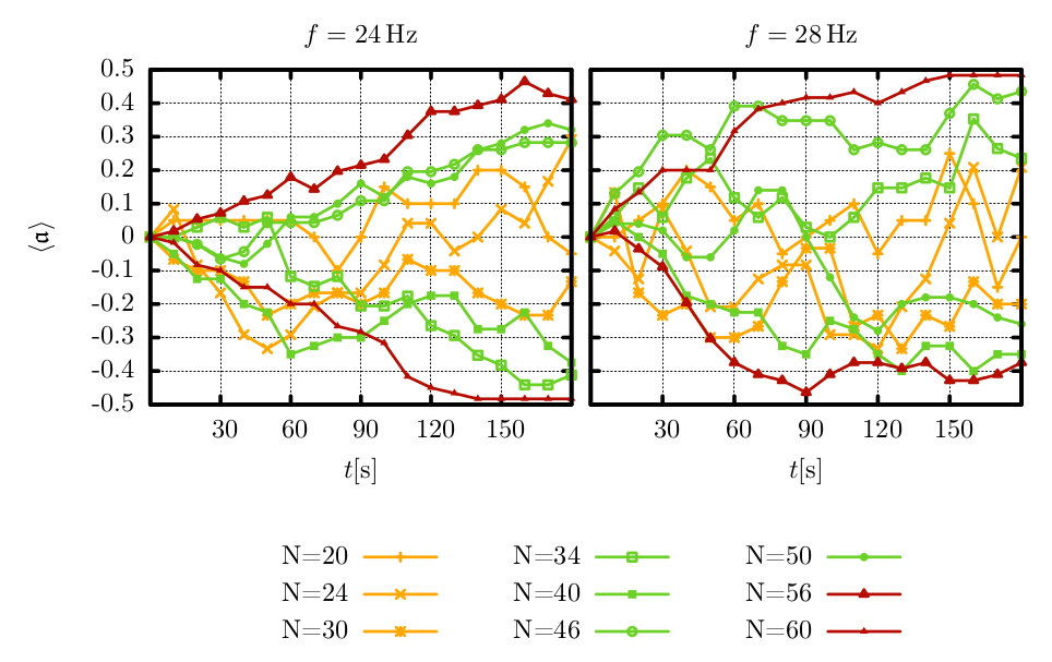
As it can be seen in the figure, the time evolution can roughly be classified into three areas:
- large values of $\boldsymbol{\mu}$ (large $N$): After only a short period time there is an imbalance between both compartments that is caused by random fluctuations. In the following a snowball effect sets in and it is hardly possible for the particles on the denser side to reach the more dilute one (as can be recognised from the almost monotonous change of the asymmetry parameter). When all particles have accumulated on one side, saturation occurs and a stationary state of total asymmetry is reached.
- moderate values of $\boldsymbol{\mu}$ (moderate $N$): After a rather chaotic initial behaviour dominated by random fluctuations the particles slowly start to cluster in of the compartments. But in comparison to the previous case the time evolution is slightly more irregular which means that from time to time particles manage to escape from the denser compartment into the more dilute one. But eventually a dynamic equilibrium is reached as well which can be thought of as stationary (except for moderate fluctuations) even though there is no total asymmetry ($\left| \mathfrak{a} \right| \approx 0.25-0.45$).
- small values of $\boldsymbol{\mu}$ (small $N$): These systems are characterised by a very irregular behaviour. Even though the system still shows a tendency to form clusters, it is unable to maintain them. Even when it succeeds in producing a significant asymmetry, it breaks up again after some time because it is not able to resist the permanent shaking. It is hardly possible for the system to reach values of $\mathfrak{a} > 3$.
Variation of the Frequency
For larger frequencies $f$ but fixed particle numbers $N$ the mean kinetic energy is larger which gives rise to a higher particle flux across the mid-wall. This circumstance has mainly two effects, namely an accelerated clustering (the stationary state is reached earlier) and a higher fluctuation (a more irregular behaviour).
Bifurcation
Variation of the Particle Number
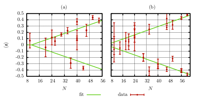
The previous figure shows the dependence of $\langle \mathfrak{a} \rangle$ on the particle number $N$. Figure (a) shows the dependence for a configuration with the high wall [height $h_h=38.0 \pm 0.1 \,\text{cm}$] and a frequency $f=32\,\text{Hz}$. Figure (b) shows the same dependence for a configuration with the low wall [height $h_l = 31.0 \pm 0.1 \,\text{cm}$] and a frequency $f=24\,\text{Hz}$. According to the theory a linear dependence $\langle \mathfrak{a} \rangle (N)$ is expected. The fit is done by gnuplot via $f(x) = a(x-N_0)$. For values below the zero of $f$ the asymmetry parameter is assumed to vanish, so the fit is set to zero at $f(x)<0$. The resulting bifurcation curve is expected to be symmetric so the fit can be done with $|\langle \mathfrak{a} \rangle|$ as parameter and then be mirrored. According to gnuplot the resulting fit parameters are
- $a=0.009(3)$, $N_0=11(7)$ for the high-wall-configuration and
- $a=0.008(2)$, $N_0=5(6)$ for the low-wall-configuration.
$N_0$ can be interpreted as the minimum particle number where asymmetric equilibrium states become possible for a given system. The apparatus was slightly oblique in the beginning. So the clustering happened to occur almost always on the same side of the wall. Fortunately, as the order of obliquity was very small, it can be justified that the clustering behaviour of the system is untouched with the exception that one side is preferred (see (a)). For the measurements illustrated in figure (b) the obliquity was corrected. As visible the assumed symmetry of the pitchfork bifurcation, i.e. the symmetry between negative and positive $\langle \mathfrak{a} \rangle$, is satisfied.
Variation of the Frequency
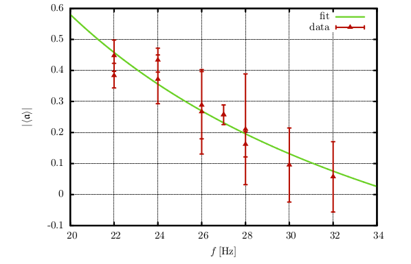
The graph shows the dependence of $|\langle \mathfrak{a} \rangle|$ of the frequency for a configuration with the low wall [$h_l=31.0 \pm 0.1 \,\text{cm}$] and $N=30$ particles. Like in the above figure (a) there occurred the problem with the slight obliquity. As according to the theory we expect a $\frac{1}{f}$ dependence of $\langle \mathfrak{a} \rangle$ the fit was done by \texttt{gnuplot} via $f(x) = \frac{1}{ax}+b$. The fit parameters turn out to be $a=0.037(4)$ and $b=-0.8(1)$.
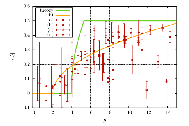
Overview of all Measurements / Variation of $\boldsymbol{\mu}$