Simulation Results
Animated Visualisation
Bifurcation
Variation of the Driving Frequency
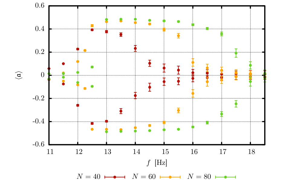
The previous figure shows our simulation results for varied driving frequency. The right hand side of the diagram includes pitchfork bifurcations. High driving frequencies correspond to high energy feeding at the bottom plate. We may distinguish three different regions in this diagram, which we discuss exemplary for $N = 80$:
For $f > 18 \,\text{Hz}$, the mean kinetic energy of a particle (and therefore the temperature of the system) is high enough that it is able to pass the middle wall without significant restrictions. A separation in two phases with different particle density and temperature does not happen here, the configuration is symmetric. The configuration corresponds to an isotropic gas. We may call this region the high temperature phase.
For $13 \,\text{Hz} < f < 18 \,\text{Hz}$ the bifurcation occurs, such that for decreasing driving frequency (energy) the asymmetry parameter tends to $\pm 0.5$ respectively. Here the "demon" starts to work. We explain this behaviour as follows:
Statistical fluctuations in the particle distribution in the box lead to an amount of inter particle collisions in one of the compartments.
This implies more energy dissipation and therefore a decrease of the mean kinetic energy and the temperature.
The particle flux between the two box divisions equalises over the time, such that two phases with different temperature and density are observed.
In the third region $f < 13\,\text{Hz}$ the asymmetry parameter tends back to zero for decreasing $f$. This is not correctly described by the theory, where we would expect that the asymmetry parameter stays close to 0.5.
The explanation for this untheoretical behaviour is obvious:
Since low frequency implies low energy feeding, the particles lack the necessary energy to pass the middle wall. In the limit case no particle passes the middle wall and the asymmetry parameter stays at its initial value which is about 0 for our simulation (random starting positions). We call this the low temperature phase. For $f \longrightarrow 0$ one could say that the granular gas now forms two independent solid phases.
In a whole, the graph loosely resembles the form of a pufferfish.
These qualitative characteristics do also hold for $N = 40$ and $N = 60$. The bifurcation point moves to lower frequencies for decreasing $f$. This is in consent with the theory: There the bifurcation starts for $\mu > 4$ where $\mu \propto N, \mu \propto f^{-2}$. For $f \longrightarrow \infty$, $\mu \approx 0$. For constant $f$, $\mu$ is greater for greater $N$. Thus we expect the start of the bifurcation as is in the diagram.
Furthermore, it is worth mentioning that the graph is very symmetric around the middle axis, except for some values at the lower end of the $f$-range.
Since none of the two compartments of the box is in any way advantaged, this fact matches our physical intuition well.
Variation of the Number of Particles
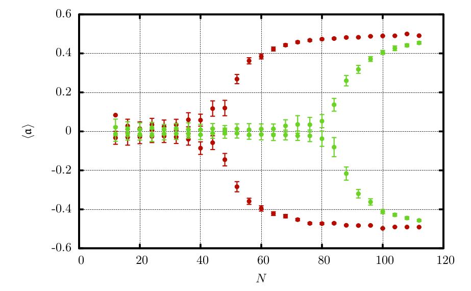
The previous figure shows the results of our simulation for varied $N$. We easily identify pitchfork bifurcations that tend to the maximal possible asymmetry parameter $\pm 0.5$.
The bifurcation point moves to greater particle numbers for increasing $f$.This coincides with the formulas of the theory section. We have already discussed these dependencies in the previous section. For small $N$, $\mu \approx 0$ and $\mu$ is greater for greater $f$ (since $v_b$ is proportional to $f$).
Variation of the Mid-Wall Height
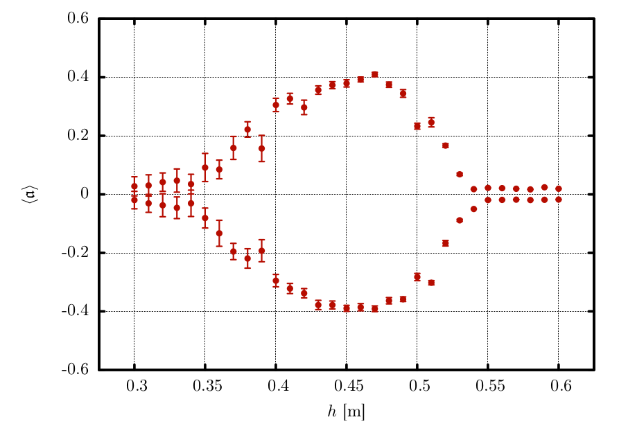
The previous figure shows the bifurcation depending on $h$. Again it has the form of a pufferfish bifurcation. The "theoretical" part of the diagram is in the region of low wall height. For small values of $h$ ($\lessapprox 0.35\,\text{m}$) $\langle \mathfrak{a} \rangle \approx 0$. Here the mean kinetic energy of the particles (and therefore their velocity) is high enough that they are able to pass the middle way without restrictions.We deduce that the particles form an isotropic gas with equal temperature and density all over the box in this region.
For $h \gtrapprox 0.35\,\text{m}$, a phase separation takes place. The particles distribute asymmetrically in the box, because the middle wall is now high enough to prevent also middle energy particles from changing the compartment and the same mechanism as described in the previous sections applies.
But for $h \gtrapprox 0.47\,\text{m}$, in contrast to the theory, the asymmetry reduces for increasing $h$. It is intuitively clear that for very high $h$ the flux between the compartments will tend to zero, since in the limit case ($h$ as high as the box) the box is completely separated into two independent parts and the particle densities stay at their initial values. The higher the wall the higher is the needed energy to fly over it. Also the range of possible angles that particles, which move from the bottom of the box to the top, need to pass the wall, decreases. This explains the pufferfish form of the data points in the diagram.
It is worth to mention, that for the parameter configuration in the last figure the asymmetry parameter does not even reach its maximal values $\pm 0.5$, but has its maximum around $\pm 0.4$. This maximal value would be greater for parameter configurations, for which the bifurcation starts earlier in terms of $h$ (see the diagrams above) since we could reckon that the flux cutoff effect described above depends less on the parameters $f$ and $N$ than the classical bifurcation (e.g. the range of possible angles is equally small for all $(f, N)$-configurations).
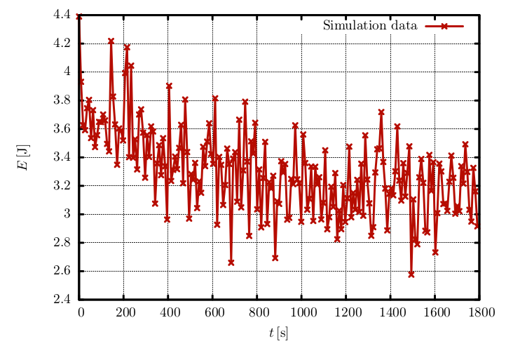
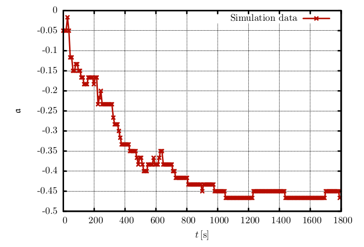
Energy and Exemplary Time Evolution